🌬️ CFD / AERODYNAMICS

3D CFD Flow Analysis on Airfoil

Examination of the three-dimensional flow field solved with ANSYS Fluent with contour planes and streamlines in CFD-Post: acceleration regions, boundary layer development and the wake region behind the trailing edge.

22.0m/s

Maximum Speed

Flow Field

Section Plane

2021 R2

ANSYS Version

📋

Project Imprint

My role	Establishing the flow solution, solving it and post-processing work
geometry	CAD geometry belongs to the project owner; flow analysis and evaluation was carried out by me
software	ANSYS Fluent 2021 R2, ANSYS Meshing, ANSYS CFD-Post
fluid	Air is assumed to be incompressible
output	Velocity magnitude contours, streamlines and section plane evaluations

🎯

Purpose and Scope

The aim of the study was to numerically solve the flow field around an airfoil and make it visible where it accelerates around the profile, where it slows down and what kind of trace it leaves behind. Since no experimental wind tunnel measurements are available, the study a qualitative flow assessment and the results were interpreted within this framework.

🌊 Solving the Velocity Field Three-dimensional solving of the velocity field around the wing and mapping of acceleration zones.	📉 Trace Zone Examining the location and width of the velocity deficit behind the trailing edge.
🔁 Methodology CAD → meshing → solution → setting up the end-to-end processing chain and making it repeatable.	👁️ Visualization Presenting the result with section planes and streamlines in a way that can be explained to a non-technical audience.

⚙️

Method Followed

Geometry Preparation

Adapting the CAD model to flow analysis: separating the solid body from the fluid volume and defining the solution space around it.

Networking

Generation of volume mesh with ANSYS Meshing; Tightening the mesh to dissolve the boundary layer in the region close to the wing surface.

Boundary Conditions and Solution

Solving the flow field with ANSYS Fluent by defining velocity at the inlet, pressure at the exit, and no-slip condition on the wing surface.

Post Processing

Three-dimensional examination of the flow field by creating section planes, velocity contours and streamlines in CFD-Post.

📊

Flow Field Evaluation

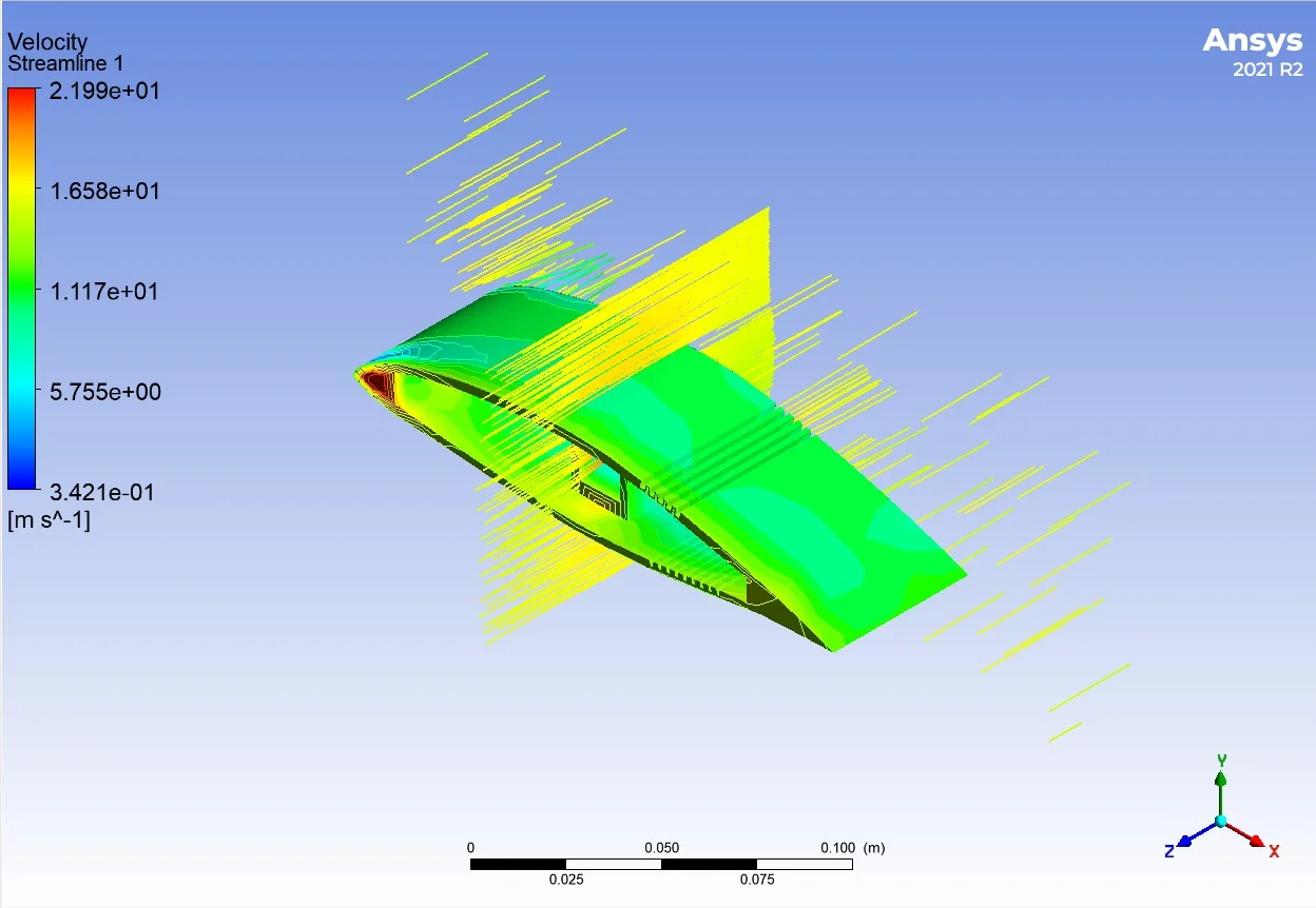
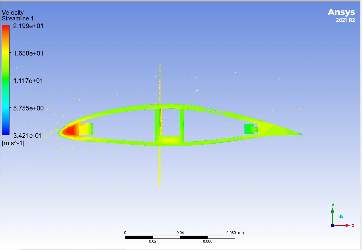
Velocity magnitude in the resolved flow field 0.34 m/s to 22.0 m/s varies in the range. The following three findings were evaluated on section planes.

Leading Edge Zone

The highest velocity values in the flow field are observed around the leading edge. The acceleration of the flow as it goes around the profile is the expected result of the cross-sectional narrowing, and this region also corresponds to the region where the pressure is lowest.

Boundary Layer Development

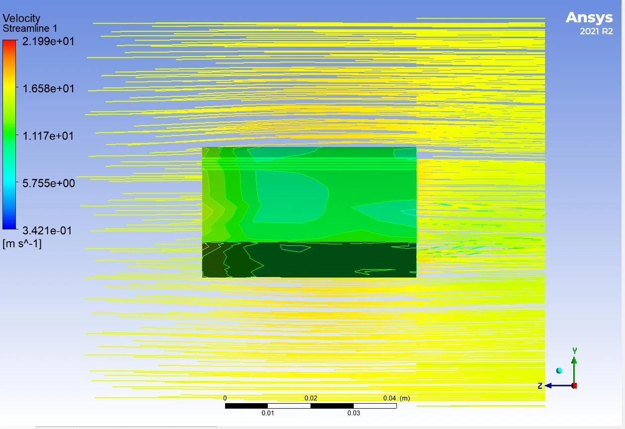
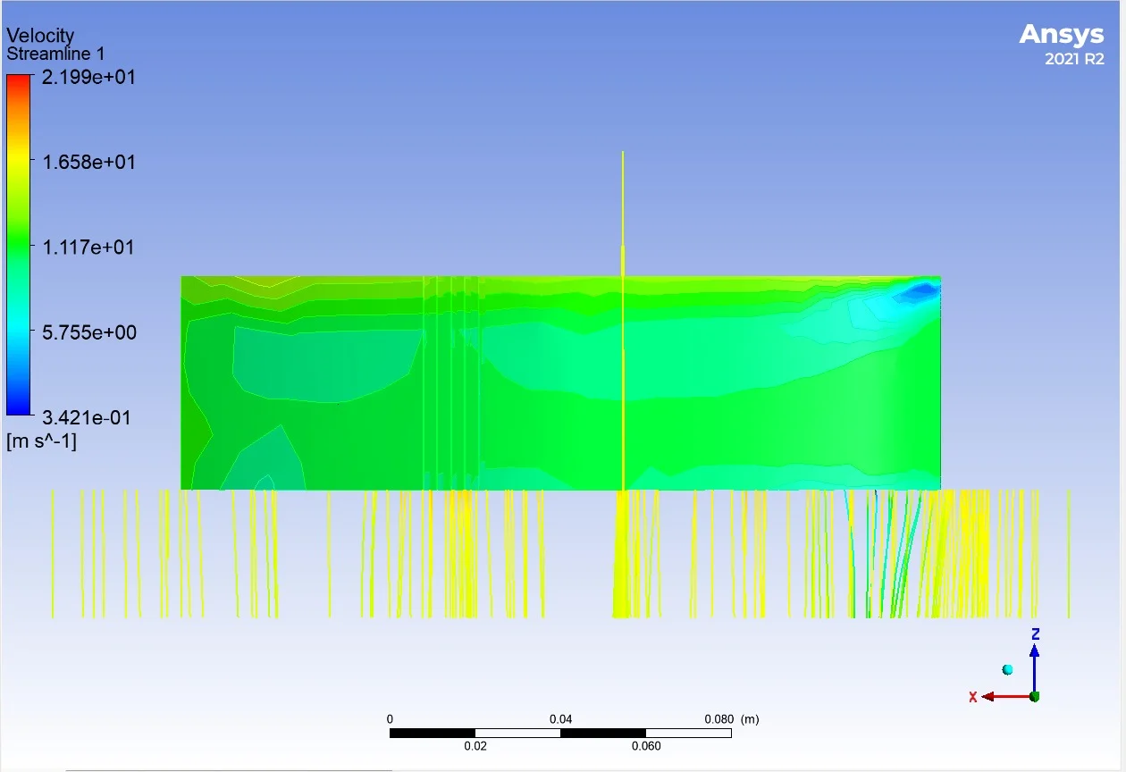
In the cross-sectional planes taken along the wing span, it is seen that the velocity in the near-surface region drops significantly below the free stream value. This is a direct indication of the boundary layer developing due to the no-slip condition at the surface, and it thickens from the root to the tip of the wing.

Trace Zone (Wake)

A region forms just behind the trailing edge where the velocity drops below the free stream value. This speed deficit is a qualitative indicator of the profile's contribution to the total drag force; The wider and deeper the wake region, the higher the resistance of the profile to flow.

🖼️

Images

40676a13-16cf-4de8-8276-0586b12abc65 — Velocity magnitude contour in profile section. The highest speed values are seen around the leading edge.

a090db27-75e0-48c0-93ef-9fc8771bf207 — Vertical section plane taken across the wingspan. It is seen that in the region close to the surface, the velocity decreases compared to the free flow and the boundary layer develops.

c376848d-5742-4a43-8c24-bd0efb7cf930 — Horizontal section plane. The low velocity area in the right region shows the wake region behind the trailing edge.

cab85d5e-b5e1-433b-9800-1a29da4fadc1 — Three-dimensional overview: wing surface, intersecting contour planes and streamlines combined.

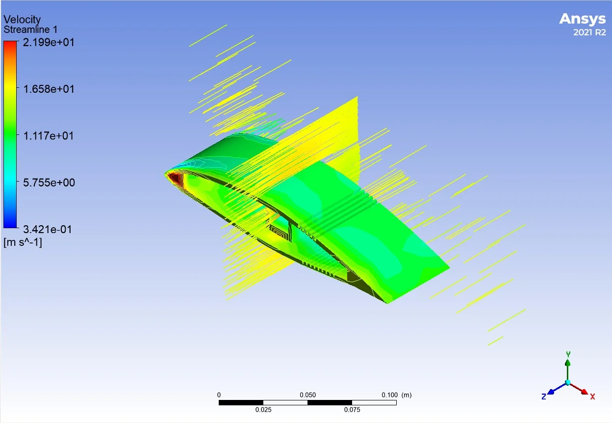
🎬 Flow Field Video

Three-dimensional examination of the resolved flow field in CFD-Post.

🔍

Limits of This Study

The value of a CFD study is not in the colorful images it produces, but in knowing under what conditions it is valid. Therefore, I clearly state the limits of the study:

⚠️ No Experimental Validation

The results have not been compared to a wind tunnel measurement or an independent reference data set. Therefore, the findings on the page qualitative flow assessment It is presented as; Absolute lift and drag coefficient claims are not made.

⚠️ Transition Effects at Model Scale

In model-scale airfoils, the flow operates in a much lower Reynolds regime than in a full-scale aircraft wing. In this regime, on the suction surface laminar separation bubbles can occur, and fully turbulent RANS models cannot capture this phenomenon; In the literature, transition sensitive models (γ-Re) for such flows_θ Transition SST, k-k_L.-ω) has been shown to be necessary. The results should be read with this limitation in mind.

✅ Next Steps

Steps planned to transform this work from a visualization to a real design tool: C with angle of attack scanning_L.–α and C_D.extraction of –α curves, documentation of mesh independence study, wall y⁺ reporting the distribution and comparing the results with XFOIL or published experimental data.

💡

Implications

1. Geometry preparation is half the solution. In external flow analysis, clean separation of the solid body from the fluid volume is more decisive than solvent settings. An unsealed surface leads to fluid meshing of internal spaces, resulting in physically meaningless results.

2. Model selection depends on the regime. Different turbulence and transition models are required for the same geometry at different Reynolds numbers. The “choose default model and move on” approach introduces systematic error in model-scale flows.

3. An unverified result is no result. Contour images are convincing, but alone they do not form the basis for engineering decisions. Next to each numerical result, the assumptions on which it was produced and where it becomes obsolete should be written.

Software and methods used within the scope of this project:

ANSYS Fluent ANSYS Meshing CFD-Post aerodynamics Boundary Layer Fluid Mechanics

3D CFD Flow Analysis on Airfoil (ANSYS Fluent)